2-D Fitting in Sherpa
Fit image data of a supernova remnant G21.5-0.9 using a 2-D multi-component
source model. First, download the FITS image of G21.5-0.9
and start IPython:
$ ipython --matplotlib
Do the usual imports of numpy and matplotlib:
import numpy as np
import matplotlib.pyplot as plt
If you have trouble accessing the image you can download it straight away using Python:
from astropy.extern.six.moves.urllib import request
url = "http://python4astronomers.github.com/_downloads/image2.fits"
open("image2.fits", "wb").write(request.urlopen(url).read())
ls
Here we eschew the advice of keeping modules separate and load the high-level API into the default namespace:
from sherpa.astro.ui import *
As with the 1D spectrum, we can load in the data with load_data:
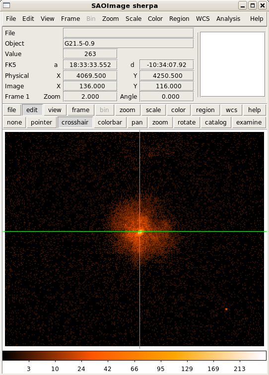
load_data("image2.fits")
print(get_data())
name      = image2.fits
x0        = Float64[56376]
x1        = Float64[56376]
y         = Float64[56376]
shape     = (216, 261)
staterror = None
syserror  = None
sky       = physical
 crval    = [ 3798.5  4019.5]
 crpix    = [ 0.5  0.5]
 cdelt    = [ 2.  2.]
eqpos     = world
 crval    = [ 278.386   -10.5899]
 crpix    = [ 4096.5  4096.5]
 cdelt    = [-0.0001  0.0001]
 crota    = 0
 epoch    = 2000
 equinox  = 2000
coord     = logical
Note
The screen output from the get_data command will depend on
whether you are using the standalone Sherpa (PyFITS) or the CIAO
version (pyCrates).
image_data()
Note
The image_data command uses ds9 to view the data rather than
matplotlib (or ChIPS).
Calculate the number of source counts in the full FOV:
calc_data_sum2d()
Result
32300
Typically, X-ray data from Chandra contain low counts, so we will switch over to a maximum likelihood statistic such as Cash:
set_stat("cash")
Note
The list_stats routine returns a list of available statistic methods.
The default fitting method, least squares, is not suitable for fitting low-count data such as X-ray images, so we will choose Simplex as the optimization method:
set_method("simplex")
Note
The list_methods routine returns the names of optimisation
methods that Sherpa provides. I also will sometimes use the
LevMar optimiser to start a fit using Cash statistics and then
switch to Simplex to check; this is not guaranteed to be any
faster or reliable!
Set the coordinate system for this image to use physical coordinates with
set_coord (Chandra chip coordinates). Valid coordinate systems include
image, physical, and wcs:
set_coord("physical")
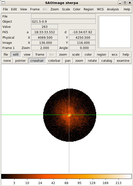
Next, we will setup a 2-D region to filter the image. Here we define a 2-D CIRCLE with x and y defined in physical coordinates and the radius defined in pixels:
notice2d("CIRCLE(4072.46,4249.34,108)")
print(get_filter())
Result
Circle(4072.46,4249.34,108)
Important
The coordinate system of the data must match the coordinate system used in
the 2-D region definition. Typically, a call to set_coord is made before
using notice2d or ignore2d.
Sherpa also supports 2-D regions from file (either ASCII or FITS).
Sherpa supports CIAO region files to define 2-D noticed regions:
ignore2d()
f = file("circle.reg", "w")
f.write("CIRCLE(4072.46,4249.34,108)\n")
f.close()

notice2d("circle.reg")
View the filtered image data in DS9:
image_data()
Hint
If you know you are not going to be using most of the image, then
filter the data before reading it into Sherpa (in CIAO you can add a
filter to the filename in the load_data command). The less data
read in can lead to quicker fits (this is generally only relevant
when you include a convolution component).
Calculate the source counts inside the noticed 2-D region:
calc_data_sum2d("CIRCLE(4072.46,4249.34,108)")
Result
24658.0
Define a 2-D Gaussian as the source model. This example is simply an illustration for describing the source emission. Initialize the parameter values according to coordinate system. The xpos and ypos parameters are in physical coordinates:
set_source(gauss2d.g1)
g1.ampl = 20
g1.fwhm = 20
g1.xpos = 4065.5
g1.ypos = 4250.5
Next, constraint the parameter limits to roughly the size of the image:
g1.fwhm.max = 4300
g1.xpos.max = 4300
g1.ypos.max = 4300
g1.ampl.min = 1
g1.ampl.max = 1000
Hint
In this case the guess command is quicker, although the limits
are not exactly the same.
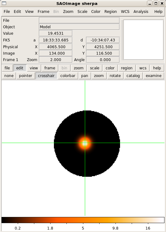
View the current model definition and view the 2-D Gaussian in DS9:
print(get_source())
gauss2d.g1
   Param        Type          Value          Min          Max      Units
   -----        ----          -----          ---          ---      -----
   g1.fwhm      thawed           20  1.17549e-38         4300
   g1.xpos      thawed       4065.5 -3.40282e+38         4300
   g1.ypos      thawed       4250.5 -3.40282e+38         4300
   g1.ellip     frozen            0            0        0.999
   g1.theta     frozen            0            0      6.28319    radians
   g1.ampl      thawed           20            1         1000

image_model()
Calculate the Gaussian model counts inside the noticed 2-D region:
calc_model_sum2d("CIRCLE(4072.46,4249.34,108)")
Result
2266.1800709135932
Now, include a background component to the source model. In this case, an estimate of (0.2) is made from a radial profile (not shown here):
set_source(g1+const2d.bgnd)
bgnd.c0 = 0.2
bgnd.c0.max = 100
View the updated model expression:
print(get_source())
(gauss2d.g1 + const2d.bgnd)
   Param        Type          Value          Min          Max      Units
   -----        ----          -----          ---          ---      -----
   g1.fwhm      thawed           20  1.17549e-38         4300
   g1.xpos      thawed       4065.5 -3.40282e+38         4300
   g1.ypos      thawed       4250.5 -3.40282e+38         4300
   g1.ellip     frozen            0            0        0.999
   g1.theta     frozen            0            0      6.28319    radians
   g1.ampl      thawed           20            1         1000
   bgnd.c0      thawed          0.2            0          100
NOTE: The function get_model is not synonymous to get_source.
Typically, Sherpa functions that end in _source refer to unconvolved model
components (e.g. components to be convolved with a Point Spread Function
(PSF)). Sherpa functions that end in _model access the complete convolved
model expression including any convolution components (e.g. PSF).
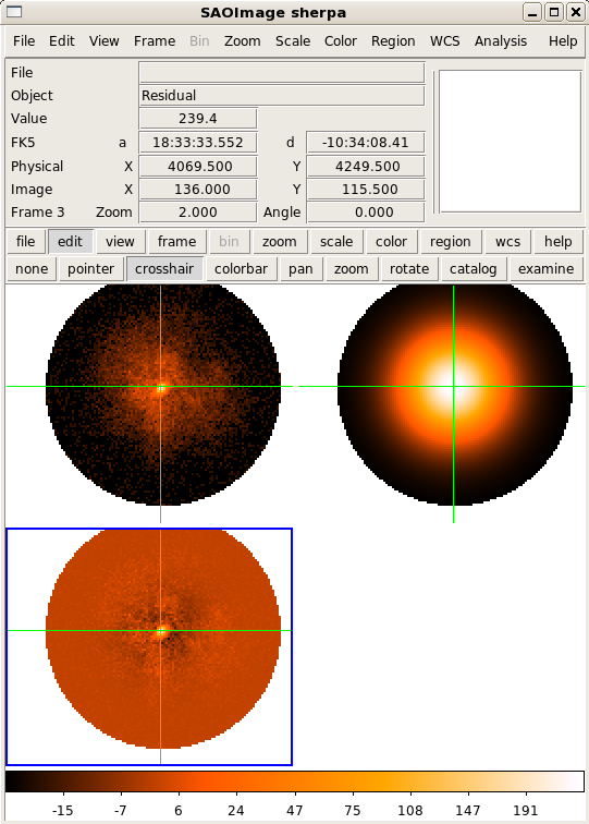
Fit with fit and display the data, model, and residuals in DS9 with
image_fit:
fit()
Dataset               = 1
Method                = neldermead
Statistic             = cash
Initial fit statistic = 20661.5
Final fit statistic   = -48907.8 at function evaluation 525
Data points           = 9171
Degrees of freedom    = 9166
Change in statistic   = 69569.3
   g1.fwhm        57.9477
   g1.xpos        4070.4
   g1.ypos        4251.11
   g1.ampl        23.3562
   bgnd.c0        0.266365

image_fit()
Fit Result
Sherpa fit results include the statistic and method used during fitting, goodness-of-fit indicators, the number of function evaluations computed, and the list of best-fit parameter values. NOTE: only the thawed parameters are shown.
Calculate the model counts inside the noticed 2-D region using the best-fit parameter values:
calc_model_sum2d("CIRCLE(4072.46,4249.34,108)")
Result
24658.000000637512
Calculate the FWHM in arcseconds using the ACIS conversion factor by accessing
the parameter value (remembering to use the the val attribute):
g1.fwhm.val * 0.492
Result
28.510281281152213
Save the fitted model to a FITS image using save_model and save the fit
residuals using save_resid:
save_model("model.fits", clobber=True)
save_resid("resid.fits", clobber=True)
Calculate the parameter confidence limits on thawed parameter values using the
Sherpa method conf, changing the range from 1 sigma (the default)
to 90 % (1.64 sigma for one interesting parameter):
set_conf_opt("sigma", 1.6448536269514722)
conf()
Confidence Result
Sherpa confidence results include the statistic and method used during, a list of best-fit parameter values, and their associated confidence limits. NOTE: only the thawed parameters or specified parameters are shown.
g1.ampl lower bound:    -0.399122
g1.fwhm lower bound:    -0.465406
g1.ampl upper bound:    0.405767
g1.fwhm upper bound:    0.467569
bgnd.c0 lower bound:    -0.0152336
g1.xpos lower bound:    -0.297327
g1.xpos upper bound:    0.297382
g1.ypos lower bound:    -0.294267
g1.ypos upper bound:    0.294294
bgnd.c0 upper bound:    0.0156245
Dataset               = 1
Confidence Method     = confidence
Iterative Fit Method  = None
Fitting Method        = neldermead
Statistic             = cash
confidence 1.64485-sigma (90%) bounds:
Param            Best-Fit  Lower Bound  Upper Bound
=====            ========  ===========  ===========
g1.fwhm           57.9477    -0.465406     0.467569
g1.xpos            4070.4    -0.297327     0.297382
g1.ypos           4251.11    -0.294267     0.294294
g1.ampl           23.3562    -0.399122     0.405767
bgnd.c0          0.266365   -0.0152336    0.0156245
Exercise (for the interested reader): SciPy special functions
Sherpa does not yet support the feature to indicate the confidence as a percentage. How can we convert the desired percentage to the sigma that Sherpa supports?
(Hint): Try scipy.special.erfinv
Click to Show/Hide Solution
Typically, the confidence is calculated from sigma using the error-function, ERF(sigma/SQRT(2)). We can invert this operation using the inverse error-function found in SciPy in the special functions module:
import scipy.special
print(scipy.special.erfinv(0.90) * numpy.sqrt(2))
Notice how the parameter confidence limits are displayed as soon as they are
known. The parameter confidence limits are accessed using get_conf_results.
Save the 90% calculated parameter limits:
results = get_conf_results()
f = file("fit_results.out", "w")
f.write("NAME VALUE MIN MAX\n")
for name, val, minval, maxval in zip(results.parnames,results.parvals,results.parmins,results.parmaxes):
    line = [name, str(val), str(val+minval), str(val+maxval)]
    print(line)
    f.write(" ".join(line)+"\n")

f.close()
View the new output file:
!cat fit_results.out
NAME VALUE MIN MAX
g1.fwhm 57.9477261812 57.4823204857 58.4152947363
g1.xpos 4070.40148441 4070.10415775 4070.69886665
g1.ypos 4251.10566089 4250.811394 4251.39995481
g1.ampl 23.3562056688 22.9570833968 23.761972516
bgnd.c0 0.266364723807 0.25113117078 0.281989200833
Notice how the function zip rotates the list of tuples into rows of names,
values, min values, and max values:
tbl = zip(results.parnames,results.parvals,results.parmins,results.parmaxes)
print(tbl[0])
('g1.fwhm', 57.947726181203684, -0.46540569551049771, 0.46756855511208073)
name, val, minval, maxval = tbl[0]
minval
-0.46540569551049771
Hint
You could use min and max as the variable names, but then
you overwrite the Python functions which can cause surprising
results later on in your session.