1-D data with errors
Here we are going to fit a 1-D spectrum with errors, so our input will be three arrays: x values, y values, and errors on the y values.
In a new working directory, download a MAST spectrum of 3C 273
and start IPython
$ ipython --matplotlib
If you have trouble accessing the spectrum you can download it straight away using Python
from astropy.extern.six.moves.urllib import request
url = 'http://python4astronomers.github.com/_downloads/3c273.fits'
open('3c273.fits', 'wb').write(request.urlopen(url).read())
We also need to load in Sherpa
import sherpa.ui as ui
import numpy as np
Loading the data
ui.load_data('3c273.fits')
print(ui.get_data())
name      = 3c273.fits
x         = Float64[1024]
y         = Float64[1024]
staterror = None
syserror  = None
Note
The load_data command may not work in the stand-alone version of
Sherpa. If not, you can use astropy.io.fits to load in the data and then
load_arrays, for example:
from astropy.io import fits
dat = fits.open('3c273.fits')[1].data
wlen = dat.field('WAVELENGTH')
flux = dat.field('FLUX')
ui.load_arrays(1, wlen, flux)
As the file contains two columns, they are taken to be the x and
y data values. The y values are small (of order 10^-14):
ui.get_data().y.mean()
4.3317031058773416e-14
np.ptp(ui.get_data().y)
9.1256637866471944e-14
Note
The numpy ptp routine returns the range of the data, and is short for “peak to peak”.
Re-scaling the data
Whilst Sherpa can deal with small (and large) values, it can be visually easier to deal with values closer to unity, so we re-scale the data values:
d1 = ui.get_data()
d1.y *= 1e14
Note
I am taking advantage of Sherpa’s use of python objects to directly change the y values of the data.
and add in errors (for the sake of this example we assume a 2 percent error on each data point).
d1.staterror == None
True
ui.set_staterror(0.02, fractional=True)
d1.staterror == None
False
ui.plot_data()
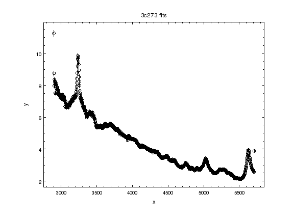
Hint
I could have used d1.staterror = 0.02 * d1.y instead of the
set_staterror command.
Note
Sherpa supports both statistical and systematic errors. Here we will be dealing with statistical errors only.
Filtering the data
It can be useful to only fit a subset of the data - e.g. to
concentrate on a particular feature - and then go back and fit
all the data. The Sherpa commands are notice and ignore.
ui.notice(3000, 5700)
From this point the extra data will not be used by Sherpa, whether in a fit or a plot command.
Hint
Try ui.plot_data() and compare the results to the original plot.
Fitting the continuum
We start with a powerlaw model, with a normalization defined at 4000 Angstroms.
ui.set_source(ui.powlaw1d.pow1)
pow1.ref = 4000.0
print(pow1)
powlaw1d.pow1
   Param        Type          Value          Min          Max      Units
   -----        ----          -----          ---          ---      -----
   pow1.gamma   thawed            1          -10           10
   pow1.ref     frozen         4000 -3.40282e+38  3.40282e+38
   pow1.ampl    thawed            1            0  3.40282e+38
Check the statistic:
ui.get_stat()
Chi Squared with Gehrels variance
ui.get_stat_name()
'chi2gehrels'
Since we have explicitly given an error column all the chi-square statistics will give the same result (the Gehrels part of the name is used to indicate how errors are estimated from the data).
ui.fit()
Dataset = 1
Method = levmar
Statistic = chi2gehrels
Initial fit statistic = 1.41325e+06
Final fit statistic = 20230.3 at function evaluation 16
Data points = 983
Degrees of freedom = 981
Probability [Q-value] = 0
Reduced statistic = 20.6221
Change in statistic = 1.39302e+06
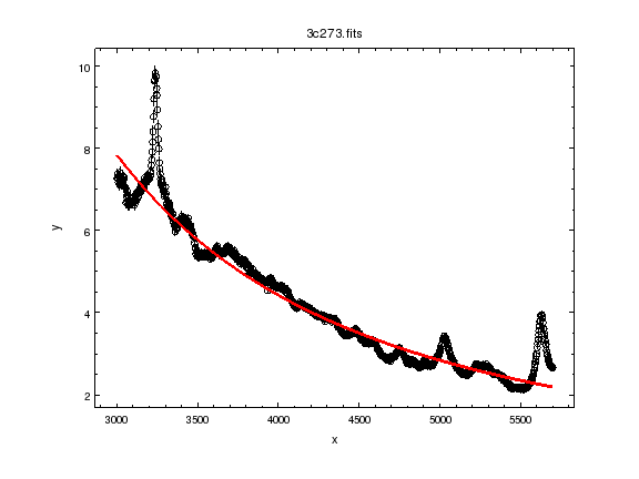
pow1.gamma 1.98798
pow1.ampl 4.42533
ui.plot_fit()
Viewing the results
results = ui.get_fit_results()
print(results)
datasets       = (1,)
itermethodname = none
methodname     = levmar
statname       = chi2gehrels
succeeded      = True
parnames       = ('pow1.gamma', 'pow1.ampl')
parvals        = (1.9879834342270963, 4.4253291641631725)
statval        = 20230.3241618
istatval       = 1413250.24877
dstatval       = 1393019.92461
numpoints      = 983
dof            = 981
qval           = 0.0
rstat          = 20.6221449152
message        = successful termination
nfev           = 16
or we can use the show_fit command, which pipes information
through a pager (typically less or more).
ui.show_fit()
Hint
There are number of show_* commands; try tab completion to
find them all.
Adding lines to the fit
I have decided to include 4 gaussians to deal with the strongest lines in the spectrum:
for n in range(1, 5):
    ui.create_model_component("gauss1d", "g{}".format(n))

ui.set_source(pow1 + g1 + g2 + g3 + g4)
ui.get_source()
<BinaryOpModel model instance '((((powlaw1d.pow1 + gauss1d.g1) + gauss1d.g2) + gauss1d.g3) + gauss1d.g4)'>
Note
I could just have included the components in the set_source
expression directly: e.g. set_source(pow1 + ui.gauss1d.g1 + ..).
Manual selection for the starting point suggests:
g1.pos = 3250
g2.pos = 5000
g3.pos = 5260
g4.pos = 5600
Note
I could also set the min/max values for these parameters to ensure
they remain in a valid range: for example ui.set_par(g1.pos, 3250, min=3000, max=5700).
We also shift the starting value for the FWHM:
for p in [g1, g2, g3, g4]:
    p.fwhm = 50
Note
Since the parameters are just Python objects we can pass them around as we would other objects.
Note
We do not use guess here since it is not designed to work on
multi-copmponent data: all the gaussians would be centered at
a wavelength of 3240.
ui.fit()
Dataset               = 1
Method                = levmar
Statistic             = chi2gehrels
Initial fit statistic = 19336.7
Final fit statistic   = 4767.96 at function evaluation 196
Data points           = 983
Degrees of freedom    = 969
Probability [Q-value] = 0
Reduced statistic     = 4.92049
Change in statistic   = 14568.7
   pow1.gamma     2.10936
   pow1.ampl      4.34391
   g1.fwhm        40.2425
   g1.pos         3239.92
   g1.ampl        2.81148
   g2.fwhm        68.9131
   g2.pos         5032.03
   g2.ampl        0.677329
   g3.fwhm        129.595
   g3.pos         5280.45
   g3.ampl        0.304465
   g4.fwhm        78.9905
   g4.pos         5634.3
   g4.ampl        1.61164

ui.plot_fit_delchi()
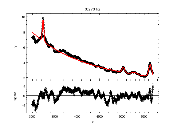
Hint
Since we have errors we can now look at the residuals in terms of ‘sigma’.
More gaussians
I want to know if there’s a broad-line component for the 3240 Angstrom line, and I want to show you how to “link” model parameters, so I will assume that the broad-line component has four times the width of the narrow component.
ui.gauss1d.g1broad
<Gauss1D model instance 'gauss1d.g1broad'>
g1broad.pos = g1.pos
g1broad.fwhm = g1.fwhm * 4
ui.set_source(ui.get_source() + g1broad)
Note
You can create model components whenever you want; it need
not be within a set_source call. Similarly, source expressions
can be treated as a variable.
print(ui.get_source())
(((((powlaw1d.pow1 + gauss1d.g1) + gauss1d.g2) + gauss1d.g3) + gauss1d.g4) + gauss1d.g1broad)
   Param        Type          Value          Min          Max      Units
   -----        ----          -----          ---          ---      -----
   pow1.gamma   thawed      2.10936          -10           10
   pow1.ref     frozen         4000 -3.40282e+38  3.40282e+38
   pow1.ampl    thawed      4.34391            0  3.40282e+38
   g1.fwhm      thawed      40.2425  1.17549e-38  3.40282e+38
   g1.pos       thawed      3239.92 -3.40282e+38  3.40282e+38
   g1.ampl      thawed      2.81148 -3.40282e+38  3.40282e+38
   g2.fwhm      thawed      68.9131  1.17549e-38  3.40282e+38
   g2.pos       thawed      5032.03 -3.40282e+38  3.40282e+38
   g2.ampl      thawed     0.677329 -3.40282e+38  3.40282e+38
   g3.fwhm      thawed      129.595  1.17549e-38  3.40282e+38
   g3.pos       thawed      5280.45 -3.40282e+38  3.40282e+38
   g3.ampl      thawed     0.304465 -3.40282e+38  3.40282e+38
   g4.fwhm      thawed      78.9905  1.17549e-38  3.40282e+38
   g4.pos       thawed       5634.3 -3.40282e+38  3.40282e+38
   g4.ampl      thawed      1.61164 -3.40282e+38  3.40282e+38
   g1broad.fwhm linked       160.97      expr: (g1.fwhm * 4)
   g1broad.pos  linked      3239.92             expr: g1.pos
   g1broad.ampl thawed            1 -3.40282e+38  3.40282e+38
Note
The parameter values indicate when they are linked, and to what, in the output above.
Since I am interested in the first line, and the other lines are unlikely to change the fit significantly, we freeze them:
ui.freeze(g2, g3, g4)
and filter out parts of the data that “look messy” (e.g. the Fe complex).
ui.ignore(3360, 4100)
ui.fit()
Dataset               = 1
Method                = levmar
Statistic             = chi2gehrels
Initial fit statistic = 4802.25
Final fit statistic   = 2307.19 at function evaluation 92
Data points           = 714
Degrees of freedom    = 708
Probability [Q-value] = 2.14817e-168
Reduced statistic     = 3.25874
Change in statistic   = 2495.06
   pow1.gamma     2.01481
   pow1.ampl      4.22548
   g1.fwhm        28.882
   g1.pos         3239.96
   g1.ampl        2.26982
   g1broad.ampl   1.0672

ui.plot_fit_delchi()

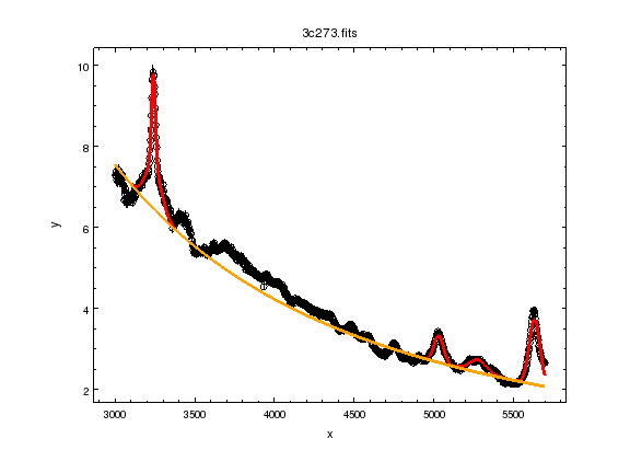
Now we add back in the “ugly” part of the spectrum and plot up the contribution from just the power-law component.
ui.notice(3000, 5700)
ui.plot_fit()
ui.plot_model_component(pow1, overplot=True)
What about errors?
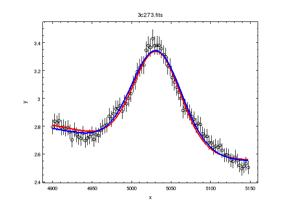
It is no good just being able to fit parameter values, we want to know errors on these values. Since the overall fit is not particularly good (a reduced chi-square of over 3), here I focus on a single line:
ui.notice()
ui.notice(4900, 5150)
ui.plot_fit()
Note
The notice and ignore commands behave differently
when no previous filter has been applied to when they are being
used to adjust a previously-filtered data set.
Here we fit just the g2 and pow1 components:
ui.freeze(g1, g1broad, g3, g4)
ui.thaw(g2)
ui.fit()
Dataset               = 1
Method                = levmar
Statistic             = chi2gehrels
Initial fit statistic = 45.9588
Final fit statistic   = 38.8045 at function evaluation 37
Data points           = 91
Degrees of freedom    = 86
Probability [Q-value] = 0.999997
Reduced statistic     = 0.451215
Change in statistic   = 7.15427
   pow1.gamma     1.90087
   pow1.ampl      4.0954
   g2.fwhm        73.7743
   g2.pos         5031.71
   g2.ampl        0.69471

ui.plot_model(overplot=True)
# pychips.set_curve(['*.color', 'blue'])
The reduced chi-square value is significantly less than 1, which suggests that the errors have been over-estimated, but let’s continue with the analysis:
ui.get_fit_results().rstat
0.45121542024712424
ui.conf()
pow1.gamma lower bound:       -0.165746
g2.pos lower bound:   -0.937708
g2.pos upper bound:   0.937708
pow1.gamma upper bound:       0.165746
g2.ampl lower bound:  -0.0189111
g2.ampl upper bound:  0.0189111
pow1.ampl lower bound:        -0.149452
pow1.ampl upper bound:        0.154944
g2.fwhm lower bound:  -2.71108
g2.fwhm upper bound:  2.80876
Dataset               = 1
Confidence Method     = confidence
Iterative Fit Method  = None
Fitting Method        = levmar
Statistic             = chi2gehrels
confidence 1-sigma (68.2689%) bounds:
   Param            Best-Fit  Lower Bound  Upper Bound
   -----            --------  -----------  -----------
   pow1.gamma        1.90087    -0.165746     0.165746
   pow1.ampl          4.0954    -0.149452     0.154944
   g2.fwhm           73.7743     -2.71108      2.80876
   g2.pos            5031.71    -0.937708     0.937708
   g2.ampl           0.69471   -0.0189111    0.0189111
Note
It should hopefully come as no suprise to find out that there is
a get_conf_results command that returns the conf results
as a Python object.
Hint
The covar command can also be used; for a good search space
it should return the same results, but is not as robust for
more-complicated situations.
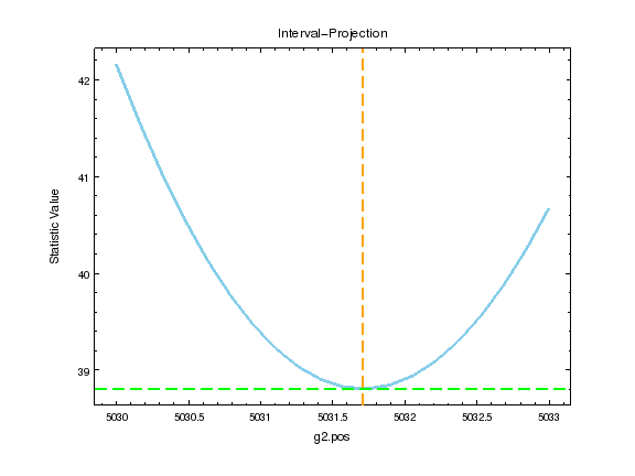
We can look at the search surface for one or two parameters with
the int_proj and reg_proj commands:
ui.int_proj(g2.pos)
ui.int_proj(g2.pos, min=5030, max=5033)
Note
int_proj is short for interval projection, and reg_proj
stands for region projection. Both commands create a plot showing
how the statistic value changes as the parameter(s) vary (by
re-fitting all the other thawed parameters).
ui.reg_proj(g2.fwhm, pow1.gamma)
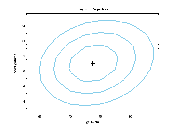
Note
The error routines - e.g. conf, int_proj, and reg_proj -
will take advantage of multiple cores on your machine. Unfortunately
fit does not.