Astropy II: Analyzing UVES Spectroscopy

This tutorial follows my real live data analysis of MN Lup and the code developed below is taken (with only minor modifications) from the code that I used to actually prepare the publication. The plots that will be developed below appear in very similar form in the article published in ApJ (771, 70, 2013).

The examples below depend on each other and the plots in the last section make use of things calculated in the earlier sections. Thus, if you need to restart your python session in the course of this tutorial, please execute all the code again.

Also, this tutorial works best if you follow along and execute the code shown on your own computer. The page is already quite long and I do not include the output you would see on your screen in this document.

Before you proceed

Please download this this tar file and extract the content, either by clicking on the link or by executing this python code:

from astropy.extern.six.moves.urllib import request
import tarfile
url = 'http://python4astronomers.github.io/_downloads/astropy_UVES.tar.gz'
tarfile.open(fileobj=request.urlopen(url), mode='r|*').extractall()
cd UVES
ls

Then start up IPython with the --matplotlib option and do the usual imports to enable interactive plotting:

$ ipython --matplotlib

import numpy as np
import matplotlib.pyplot as plt

Acknowledgments

Authors:Moritz Guenther Copyright:2013 Moritz Guenther

Based on observations made with ESO Telescopes at the La Silla Paranal Observatory under program ID 087.V0991(A).

Scientific background

In this tutorial we analyze data from MN Lup, a T Tauri star in the Taurus-Auriga star forming region located at a distance of about 140 pc. MN Lup has been observed simultaneously with XMM-Newton and the UVES spectrograph on the VLT. MN Lup is suspected to be a classical T Tauri star, that is accreting mass from a circumstellar disk. MN Lup has been Doppler imaged by Strassmeier et al. (2005, A&A, 440, 1105) with a very similar UVES setup and those authors claim an rotationally modulated accretion spot.

In the X-ray data we find moderate indications for accretion. In this tutorial we analyze (some of) the UVES data to search for rotationally modulated features in the emission line profiles, which could be due to an accretion spot on the stellar surface.

Reading the data

The previous astropy tutorial already covered Handling FITS files and WCS Transformations, so the explanation here is only very brief. Check the astropy documentation or the other two tutorials for more details:

from glob import glob

import numpy as np

from astropy.wcs import WCS
from astropy.io import fits

# glob searches through directories similar to the Unix shell
filelist = glob('*.fits')
# sort alphabetically - given the way the filenames are
# this also sorts in time
filelist.sort()

Read the first fits file in the list and check what is in there:

sp = fits.open(filelist[0])
sp.info()

We see that the data is given as the primary image and all other info is part of the primary header. So, we can extract the WCS from that header to get the wavelength coordinate:

header = sp[0].header

wcs = WCS(header)
#make index array
index = np.arange(header['NAXIS1'])

wavelength = wcs.wcs_pix2world(index[:,np.newaxis], 0)
wavelength.shape
#Ahh, this has the wrong dimension. So we flatten it.
wavelength = wavelength.flatten()

The flux is contained in the primary image:

flux = sp[0].data

Making code reusable as a function

Now, we do not want to repeat this process for every single file by hand, so let us define a function that takes the filename as input and returns the wavelength and flux arrays and the time of the observation. In python, functions are created with the def statements. All lines that have an indentation level below the def statement are part of the function. Functions can (but do not have to) return values using the return statement.

If a function func is contained in a file called spectra_utils.py in the current directory, then this file can be imported into a python session in order to use the function func with the following command:

import spectra_utils
a = spectra_utils.func(param1, param2, ...)

Alternatively, you can import just one (or a few) of many different functions that are defined in your file spectra_utils.py:

from spectra_utils import func
a = func(param1, param2, ...)

You will recognize that python does not make a difference between modules that come with python (e.g. glob), external modules (e.g. numpy or astropy) and modules that you write yourself. The syntax to import those modules or functions is the same in all cases, provided that the directory where your module is defined is in the search path (more about python modules and the search path).

Note

You can also define a function on the interactive interpreter by just typing it line by line. However, if you work in an interactive session, then the function ends as soon as there is a blank line. This makes it a little inconvenient to copy and paste more than the simplest functions into an interpreter. Fortunately, ipython offers two magic functions that take care of this:

1. You can mark code in some editor, copy it to the clipboard and then type %paste in ipython.
2. You type %cpaste in ipython you can paste code (e.g. with the mouse) and ipython will correct the leading number of white spaces and ignore empty lines.

These two tricks can be used with any type of code, but are particularly useful to define functions.

Note

Once you used import spectra_utils python will not monitor the source file. If you change the source code of func in the file, you need to reload(spectra_utils) to load the new version of func.

So, after all this discussion, we can now define a function that automates the loading of a single spectrum using the commands we developed above. Even if this function is fairly short, we still add some documentation to the header, so that we can look up what parameters it needs when we come back to this project a while later. Personally, I comment every function that is longer than two lines:

def read_spec(filename):
    '''Read a UVES spectrum from the ESO pipeline

    Parameters
    ----------
    filename : string
       name of the fits file with the data

    Returns
    -------
    wavelength : np.ndarray
        wavelength (in Ang)
    flux : np.ndarray
        flux (in erg/s/cm**2)
    date_obs : string
        time of observation
    '''
    sp = fits.open(filename)
    header = sp[0].header

    wcs = WCS(header)
    #make index array
    index = np.arange(header['NAXIS1'])

    wavelength = wcs.wcs_pix2world(index[:,np.newaxis], 0)
    wavelength = wavelength.flatten()
    flux = sp[0].data

    date_obs = header['Date-OBS']
    return wavelength, flux, date_obs

Exercise

Try to find out how you can read the help for this function from the command line.

Click to Show/Hide Solution

help(read_spec)
#or
read_spec?

Exercise

The dataset of UVES spectra should have been taken using all the same setup. Write a function that returns the exposure time (EXPTIME), the wavelength zero point (CRVAL1), and the arm used (UVES has a red and a blue arm - see keyword HIERARCH ESO INS PATH). Then check that all exposures have the same setup.

Click to Show/Hide Solution

def read_setup(filename):
    '''Get setup for UVES spectrum from the ESO pipeline

    Parameters
    ----------
    filename : string
       name of the fits file with the data

    Returns
    -------
    exposure_time : float
    wavelength_zero_point : float
    optical_arm : string
    '''
    sp = fits.open(filename)
    header = sp[0].header

    return header['EXPTIME'], header['CRVAL1'], header['HIERARCH ESO INS PATH']

# Let's just print the setup on the screen
# We'll see if it's all the same.
for f in filelist:
    print(read_setup(f))

The UVES pipeline that was used to reduce the data that we use in the this example employs a fixed wavelength grid (see exercise above), thus the wavelength is the same for all spectra. This makes it easy to define an array that can hold the fluxes of all observations. Then, we loop over the list of all filenames and fill this array with data:

flux = np.zeros((len(filelist), len(wavelength)))
# date comes as string with 23 characters (dtype = 'S23')
date = np.zeros((len(filelist)), dtype = 'S23')

for i, fname in enumerate(filelist):
    w, f, date_obs = read_spec(fname)
    flux[i,:] = f
    date[i] = date_obs

Units and constants in astropy

Often, one has to keep track of the units for certain values. Was the wavelength given in Angstrom or in nm? In X-ray observations, a common unit of wavelength is keV. How many nm is 0.65 keV? astropy.units offers a framework that can take care of this book-keeping and propagate the units through many (but not all) mathematical operations (e.g. addition, division, multiplication). Furthermore, astropy.constants supplies the values of many physical and astronomical constants. The easiest way to attach a unit to a number is by multiplication:

import astropy.units as u
from astropy.constants.si import c, G, M_sun, R_sun

wavelength = wavelength * u.AA

# Let's define some constants we need for the exercises further down
# Again, we multiply the value with a unit here
heliocentric = -23. * u.km/u.s
v_rad = -4.77 * u.km / u.s  # Strassmeier et al. (2005)
R_MN_Lup = 0.9 * R_sun      # Strassmeier et al. (2005)
M_MN_Lup = 0.6 * M_sun      # Strassmeier et al. (2005)
vsini = 74.6 * u.km / u.s   # Strassmeier et al. (2005)
period = 0.439 * u.day      # Strassmeier et al. (2005)

inclination = 45. * u.degree # Strassmeier et al. (2005)
# All numpy trigonometric functions expect the input in radian.
# So far, astropy does not know this, so we need to convert the
# angle manually
incl = inclination.to(u.radian)

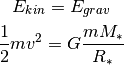
Now, we can use those variables in our calculations. MN Lup is a T Tauri star (TTS), which is possibly surrounded by an accretion disk. In the spectra we will be looking for signatures of accretion. We expect those accretion signatures to appear close to the free-fall velocity v that a mass m reaches, when it hits the stellar surface. We can calculate the infall speed using simple energy conservation:

So, let us calculate the free-fall velocity for MN Lup:

>>> v_accr = (2.* G * M_MN_Lup/R_MN_Lup)**0.5
>>> print(v_accr)
504469.027564 m / (s)
>>> # Maybe astronomers prefer it in the traditional cgs system?
>>> print(v_accr.cgs)
50446902.7564 cm / (s)
>>> # Or in some really obscure unit?
>>> print(v_accr.to(u.mile / u.hour))
1128465.07598 mi / (h)

How does the accretion velocity relate to the rotational velocity?

v_rot = vsini / np.sin(incl)
v_accr / v_rot

Oh, what is that? The seconds are gone, but astropy.quantity objects keep their different length units unless told otherwise:

(v_accr / v_rot).decompose()

The reason for this is that it is not uncommon to use different length units in a single constant, e.g. the Hubble constant is commonly given in “km/ (s * Mpc)”. “km” and “Mpc” are both units of length, but generally you do not want to shorten this to “1/s”.

We can now use the astropy.units mechanism to correct the wavelength scale to the heliocentric velocity scale:

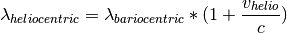
Naively, we could try:

wavelength = wavelength * (1. + heliocentric/c)
TypeError: unsupported operand type(s) for +: 'float' and 'Quantity'

However, this fails, because heliocentric/c is in units of “km/m” and 1. is just a number. From the notation above, it is not clear what we actually want. Do we ask for the value of heliocentric/c + 1. or do we want to simplify the units of heliocentric/c and after that add 1.? There are several ways to make the instruction precise, but one is to explicitly add u.dimensionless_unscaled to 1. to tell astropy that this number is dimensionless and does not carry any scaling:

wavelength = wavelength * (1. * u.dimensionless_unscaled+ heliocentric/c)

I want to mention one more feature here (check out astropy.units for more): The ability to convert the spectral axis to frequencies or energies. Normally, a unit of length is not equivalent to a unit of energy or to a frequency, but this conversion makes sense for the wavelength of a spectrum. This is how it can be done:

wavelength.to(u.keV, equivalencies=u.spectral())
wavelength.to(u.Hz, equivalencies=u.spectral())

Exercise

Spectroscopically, MN Lup is classified as spectral type M0 V, thus the gravitational acceleration on the surface should be comparable to the sun. (For non-stellar astronomers: Conventionally, all values are given in the cgs system. The value for the sun is .)

Calculate for MN Lup with the values for the mass and radius given above. Those values were determined from evolutionary tracks. Check if the is consistent with the value expected from spectroscopy.

Click to Show/Hide Solution

The values from evolutionary tracks are indeed consistent with the spectroscopically estimated surface gravity:

>>> print(np.log10((G*M_MN_Lup/R_MN_Lup**2).cgs))
4.3080943799180433

Exercise

Write a function that turns a wavelength scale into a velocity scale. We want to input a wavelengths array and the rest wavelength of a spectral line. We need this function later to show the red- and blueshift of the spectrum relative to the the Ca II H line. Use the following definition to make sure the that code below can use it later:

def wave2doppler(wavelength_array, wavelength_line):
    .. do something ..
    return array_of_dopplershifts

You can test if you function works by calculating the a Dopplershift of the following wavelengths relative to :

waveclosetoHa = np.array([6562.,6563,6565.]) * u.AA
print(wave2doppler(waveclosetoHa, 656.489 * u.nm))

I get -132, -86 and +5 km/s.

Click to Show/Hide Solution

def wave2doppler(w, w0):
    doppler = ((w-w0)/w0 * c)
    return doppler

print(wave2doppler(waveclosetoHa, 656.489 * u.nm).decompose().to(u.km/u.s))

Exercise

Write a function that takes a wavelength array and the rest wavelength of a spectral line as input, turns it into a Doppler shift (you can use the function from the last exercise), subtracts the radial velocity of MN Lup (4.77 km/s) and expresses the resulting velocity in units of vsini. We need this function later to show the red- and blueshift of the spectrum relative to the Ca II H line. Use the following definition to make sure the that code below can use it later:

def w2vsini(wavelength_array, wavelength_line):
    .. do something ..
    return array_of_shifts_in_vsini

Click to Show/Hide Solution

def w2vsini(w, w0):
    v = wave2doppler(w, w0) - 4.77 * u.km/u.s
    return v / vsini

Converting times

astropy.time provides methods to convert times and dates between different systems and formats. Since the ESO fits headers already contain the time of the observation in different systems, we could just read the keyword in the time system we like, but we will use astropy.time to make this conversion here. astropy.time.Time will parse many common input formats (strings, floats), but unless the format is unambiguous the format needs to be specified (e.g. a number could mean JD or MJD or year). Also, the time system needs to be given (e.g. UTC). Below are several examples, initialized from different header keywords:

from astropy.time import Time
t1 = Time(header['MJD-Obs'], format = 'mjd', scale = 'utc')
t2 = Time(header['Date-Obs'], scale = 'utc')

Times can be expressed in different formats:

>>> t1
<Time object: scale='utc' format='mjd' vals=55784.9749105>
>>> t1.isot
'2011-08-11T23:23:52.266'
>>> t2
<Time object: scale='utc' format='isot' vals=2011-08-11T23:23:52.266>

or be converted to a different time system:

>>> t1.tt
<Time object: scale='tt' format='mjd' vals=55784.9756765>

Times can also be initialized from arrays and we can calculate time differences:

obs_times = Time(date, scale = 'utc')
delta_t = obs_times - Time(date[0], scale = 'utc')

Now, we want to express the time difference between the individual spectra of MN Lup in rotational periods. While the unit of delta_t is days, unfortunately astropy.time.Time and astropy.units.Quantity objects do not work together yet, so we will have to convert from one to the other explicitly:

delta_p = delta_t.val * u.day / period

Normalize the flux to the local continuum

In this example we want to look at the time evolution of a single specific emission line in the spectrum. In order to estimate the equivalent width or make reasonable plots we need to normalize the flux to the local continuum. In this specific case the emission line is bright and the continuum can be described reasonably by a second-order polynomial.

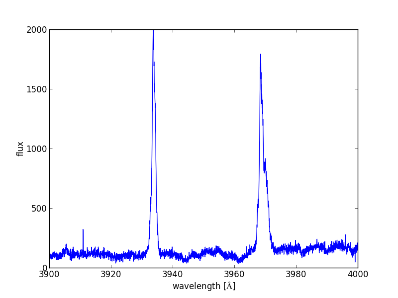
So, we define two regions left and right of the emission line, where we fit the polynomial. Looking at the figure, [3925*u.AA, 3930*u.AA] and [3938*u.AA, 3945*u.AA] seem right for that. Then, we normalize the flux by this polynomial.

The following function will do that:

def region_around_line(w, flux, cont):
    '''cut out and normalize flux around a line

    Parameters
    ----------
    w : 1 dim np.ndarray
        array of wavelengths
    flux : np.ndarray of shape (N, len(w))
        array of flux values for different spectra in the series
    cont : list of lists
        wavelengths for continuum normalization [[low1,up1],[low2, up2]]
        that described two areas on both sides of the line
    '''
    #index is true in the region where we fit the polynomial
    indcont = ((w > cont[0][0]) & (w < cont[0][1])) |((w > cont[1][0]) & (w < cont[1][1]))
    #index of the region we want to return
    indrange = (w > cont[0][0]) & (w < cont[1][1])
    # make a flux array of shape
    # (number of spectra, number of points in indrange)
    f = np.zeros((flux.shape[0], indrange.sum()))
    for i in range(flux.shape[0]):
        # fit polynomial of second order to the continuum region
        linecoeff = np.polyfit(w[indcont], flux[i, indcont],2)
        # divide the flux by the polynomial and put the result in our
        # new flux array
        f[i,:] = flux[i,indrange]/np.polyval(linecoeff, w[indrange])
    return w[indrange], f

wcaII, fcaII = region_around_line(wavelength, flux,
               [[3925*u.AA, 3930*u.AA],[3938*u.AA, 3945*u.AA]])

Publication ready output

Tables

We will calculate the equivalent width in Angstroms of the emission line for the first spectrum:

ew = fcaII[0,:] - 1.
ew = ew[:-1] * np.diff(wcaII.to(u.AA).value)
print(ew.sum())

Using numpy array notation we can actually process all spectra at once:

delta_lam = np.diff(wcaII.to(u.AA).value)
ew = np.sum((fcaII - 1.)[:,:-1] * delta_lam[np.newaxis, :], axis=1)

Now, we want to generate a LaTeX table of the observation times, period and equivalent width that we can directly paste into our manuscript. To do so, we first collect all the columns and make an astropy.table.Table object. (Please check astropy.table or Tabular data for more details on Table). So, here is the code:

from astropy.table import Column, Table
import astropy.io.ascii as ascii

datecol = Column(name = 'Obs Date', data = date)
pcol = Column(name = 'phase', data = delta_p, format = '{:.1f}')
ewcol = Column(name = 'EW', data = ew, format = '{:.1f}', units = '\\AA')
tab = Table((datecol, pcol, ewcol))
# latexdicts['AA'] contains the style specifics for A&A (\hline etc.)
tab.write('EWtab.tex', latexdict = ascii.latexdicts['AA'])

Plots

We will make two plots. The plotting is done with matplotlib, and does not involve Astropy itself. Plotting is introduced in Plotting and Images and more details on plotting can be found there. When in doubt, use the search engine of your choice and ask the Internet. Here, I mainly want to illustrate that Astropy can be used in real-live data analysis. Thus, I do not explain every step in the plotting in detail. The plots we produce below appear in very similar form in Guenther et al. 2013 (ApJ, 771, 70).

In both cases we want the x-axis to show the Doppler shift expressed in units of the rotational velocity. In this way, features that are rotationally modulated will stick out between -1 and +1:

x = w2vsini(wcaII, 393.366 * u.nm).decompose()

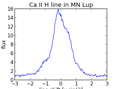
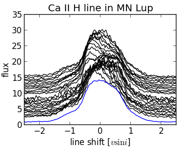
First, we will show the line profile:

import matplotlib.pyplot as plt
# set reasonable figsize for 1-column figures
fig = plt.figure(figsize = (4,3))
ax = fig.add_subplot(1,1,1)
ax.plot(x, fcaII[0,:])
ax.set_xlim([-3,+3])
ax.set_xlabel('line shift [v sin(i)]')
ax.set_ylabel('flux')
ax.set_title('Ca II H line in MN Lup')
# when using this interface, we need to explicitly call the draw routine
plt.draw()

Exercise

The plot above shows only a single spectrum. Plot all spectra into a single plot and introduce a sensible offset between them, so that we can follow the time evolution of the line.

Click to Show/Hide Solution

There are clearly several ways to produce a well looking plot. Here is one way:

yshift = np.arange((fcaII.shape[0])) * 0.5
#shift the second night up by a little more
yshift[:] += 1.5
yshift[13:] += 1

fig = plt.figure(figsize = (4,3))
ax = fig.add_subplot(1,1,1)

for i in range(25):
    ax.plot(x, fcaII[i,:]+yshift[i], 'k')

#separately show the mean line profile in a different color
ax.plot(x, np.mean(fcaII, axis =0), 'b')
ax.set_xlim([-2.5,+2.5])
ax.set_xlabel('line shift [$v \\sin i$]')
ax.set_ylabel('flux')
ax.set_title('Ca II H line in MN Lup')
fig.subplots_adjust(bottom = 0.15)
plt.draw()

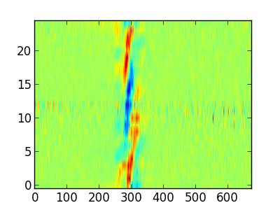
Next, we will make a more advanced plot. For each spectrum we calculate the difference to the mean flux:

fmean = np.mean(fcaII, axis=0)
fdiff = fcaII - fmean[np.newaxis,:]

In the following simple plot, we can already see features moving through the line. However, the axis scales are not right, the gap between both nights is not visible and there is no proper labeling:

fig = plt.figure(figsize = (4,3))
ax = fig.add_subplot(1,1,1)
im = ax.imshow(fdiff, aspect = "auto", origin = 'lower')

In the following, we will plot the spectra from both nights separately. Also, we will pass the extent keyword to ax.imshow which takes care of the axis:

ind1 = delta_p < 1 * u.dimensionless_unscaled
ind2 = delta_p > 1 * u.dimensionless_unscaled

fig = plt.figure(figsize = (4,3))
ax = fig.add_subplot(1,1,1)

for ind in [ind1, ind2]:
    im = ax.imshow(fdiff[ind,:], extent = (np.min(x), np.max(x), np.min(delta_p[ind]), np.max(delta_p[ind])), aspect = "auto", origin = 'lower')

ax.set_ylim([np.min(delta_p), np.max(delta_p)])
ax.set_xlim([-1.9,1.9])
plt.draw()

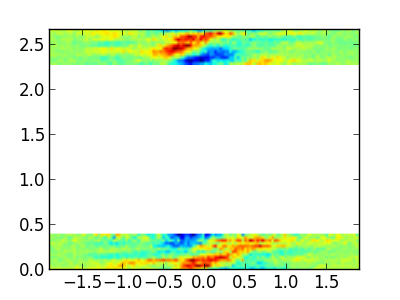
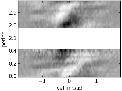
Now, this plot is already much better, but there are still some things that can be improved:

• Introduce an offset on the y-axis to reduce the amount of white space.

• Strictly speaking, the image shown is not quite the right scale because the

  extent keyword gives the edges of the image shown, while x and delta_p contain the bin mid-points.

• Use a gray scale instead of color to save publication charges.

• Add labels to the axis.

The following code addresses these points:

# shift a little for plotting purposes
pplot = delta_p.copy().value
pplot[ind2] -= 1.5
# image goes from x1 to x2, but really x1 should be middle of first pixel
delta_t = np.median(np.diff(delta_p))/2.
delta_x = np.median(np.diff(x))/2.
# imshow does the normalization for plotting really well, but here I do it
# by hand to ensure it goes -1,+1 (that makes color bar look good)
fdiff = fdiff / np.max(np.abs(fdiff))

fig = plt.figure(figsize = (4,3))
ax = fig.add_subplot(1,1,1)

for ind in [ind1, ind2]:
    im = ax.imshow(fdiff[ind,:],
         extent = (np.min(x)-delta_x, np.max(x)+delta_x,
                   np.min(pplot[ind])-delta_t, np.max(pplot[ind])+delta_t),
         aspect = "auto", origin = 'lower', cmap = plt.cm.Greys_r)

ax.set_ylim([np.min(pplot)-delta_t, np.max(pplot)+delta_t])
ax.set_xlim([-1.9,1.9])
ax.set_xlabel('vel in $v\\sin i$')
ax.xaxis.set_major_locator(plt.MaxNLocator(4))

def pplot(y, pos):
    'The two args are the value and tick position'
    'Function to make tick labels look good.'
    if y < 0.5:
        yreal = y
    else:
        yreal = y + 1.5
    return yreal

formatter = plt.FuncFormatter(pplot)
ax.yaxis.set_major_formatter(formatter)
ax.set_ylabel('period')
fig.subplots_adjust(left = 0.15, bottom = 0.15, right = 0.99, top = 0.99)
plt.draw()

Exercise

Understand the code for the last plot. Some of the commands used are already pretty advanced stuff. Remember, any Internet search engine can be your friend.

Click to Show/Hide Solution

Clearly, I did not develop this code for scratch. The matplotlib gallery is my preferred place to look for plotting solutions.

Contributing to Astropy

Astropy is an open-source and community-developed Python package, which means that is only as good as the contribution of the astronomical community. Clearly, there will always people who have more fun writing code and others who have more fun using it. However, if you find a bug and do not report it, then it is unlikely to be fixed. If you wish for a specific feature, then you can either implement it and contribute it or at least fill in a feature request.

If you want to get help or discuss issues with other Astropy users, you can sign up for the astropy mailing list. Alternatively, the astropy-dev list is where you should go to discuss more technical aspects of Astropy with the developers.

If you have come across something that you believe is a bug, please open a ticket in the Astropy issue tracker, and we will look into it promptly.

Please try to include an example that demonstrates the issue and will allow the developers to reproduce and fix the problem. If you are seeing a crash then frequently it will help to include the full Python stack trace as well as information about your operating system (e.g. MacOSX version or Linux version).

Here is a practical example. Above we calculated the free-fall velocity onto MN Lup like this:

v_accr = (2.*G *M_MN_Lup / R_MN_Lup)**0.5

Mathematically, the following statement is equivalent:

v_accr2 = np.sqrt((2.*G * M_MN_Lup/R_MN_Lup))

However, this raises a warning and automatically converts the quantity object to an numpy array and the unit is lost. If you believe that is a bug that should be fixed, you might chose to report it in the issue tracker. (But please check if somebody else has reported the same thing before, so we do not clutter the issue tracker needlessly.)