WCS Transformations
Note
If you are already familiar with PyWCS, astropy.wcs is in fact the same code as the latest version of PyWCS, and you can adapt old scripts that use PyWCS to use Astropy by simply doing:
from astropy import wcs as pywcs
However, for new scripts, we recommend the following import:
from astropy.wcs import WCS
since most of the user-level functionality is contained within the WCS class.
Documentation
For more information about the features presented below, you can read the astropy.wcs docs.
Data
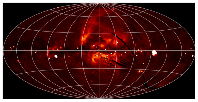
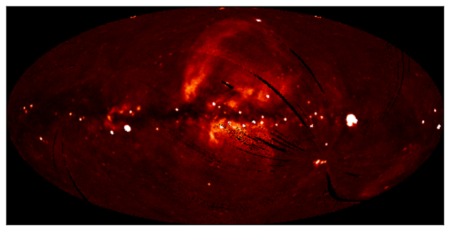
The data used in this page (ROSAT.fits) is a map of the Soft X-ray
Diffuse Background from the ROSAT XRT/PSPC in the 3/4 keV band, in an Aitoff
projection:
Representing WCS transformations
The World Coordinate System standard is often used in FITS files in order to
describe the conversion from pixel to world (e.g. equatorial, galactic, etc.)
coordinates. Given a FITS file with WCS information, such as ROSAT.fits,
we can create an object to represent the WCS transformation either by directly
supplying the filename:
>>> from astropy.wcs import WCS
>>> w = WCS('ROSAT.fits')
or the header of the FITS file:
>>> from astropy.io import fits
>>> from astropy.wcs import WCS
>>> header = fits.getheader('ROSAT.fits')
>>> w = WCS(header)
Pixel to World and World to Pixel transformations
Once the WCS object has been created, you can use the following methods to convert pixel to world coordinates:
>>> wx, wy = w.wcs_pix2world(250., 100., 1)
>>> print('{0} {1}'.format(wx, wy))
352.67460912268814 -15.413728717834152
This converts the pixel coordinates (250, 100) to the native world coordinate
system of the transformation. Note the third argument, set to 1, which
indicates whether the pixel coordinates should be treated as starting from (1,
1) (as FITS files do) or from (0, 0). Converting from world to pixel
coordinates is similar:
>>> px, py = w.wcs_world2pix(0., 0., 1)
>>> print('{0} {1}'.format(px, py))
240.5 120.5
Working with arrays
If many coordinates need to be transformed, then it is possible to use Numpy arrays:
>>> import numpy as np
>>> px = np.linspace(200., 300., 10)
>>> py = np.repeat(100., 10)
>>> wx, wy = w.wcs_pix2world(px, py, 1)
>>> print(wx)
[  31.31117136   22.6911179    14.09965438    5.52581152  356.9588445
  348.38809541  339.80285857  331.19224432  322.54503641  313.84953796]
>>> print(wy)
[-15.27956026 -15.34691039 -15.39269292 -15.4170814  -15.42016742
 -15.40196251 -15.36239844 -15.30132572 -15.21851046 -15.11362923]
Practical Exercises
Excercise 1
Try converting more values from pixel to world coordinates, and try converting these back to pixel coordinates. Do the results agree with the original pixel coordinates? Also, what are the world coordinates of the pixel at (1, 1), and why?
Click to Show/Hide Solution
The final pixel coordinates should always agree with the starting ones, since each pixel covers a unique world coordinate position. The world coordinates of the pixel at (1, 1) are not defined:
w.wcs_pix2world(1, 1, 1)
[array(nan), array(nan)]
because the pixel lies outside the coordinate grid. Thus, not all pixels in an image have a valid position on the sky.
Excercise 2
Extract and print out the values in the ROSAT map at the position of the LAT Point Sources (from the FITS tutorial)
Click to Show/Hide Solution
import numpy as np
from astropy.io import fits
from astropy.wcs import WCS
from astropy.table import Table

# Read in Point Source Catalog
data = fits.getdata('gll_psc_v08.fit',1)
psc = Table(data)

# Extract Galactic Coordinates
l = psc['GLON']
b = psc['GLAT']

# Read in ROSAT map
hdulist_im = fits.open('ROSAT.fits')

# Extract image and header
image = hdulist_im[0].data
header = hdulist_im[0].header

# Instantiate WCS object
w = WCS(header)

# Find pixel positions of LAT sources. Note we use ``0`` here for the last
# argument, since we want zero based indices (for Numpy), not the FITS
# pixel positions.
px, py = w.wcs_world2pix(l, b, 0)

# Find the nearest integer pixel
px = np.round(px).astype(int)
py = np.round(py).astype(int)

# Find the ROSAT values (note the reversed index order)
values = image[py, px]

# Print out the values
print(values)
which gives:
[ 123.7635498   163.27642822  221.76609802 ...,  255.07995605  100.35219574
   87.62506104]
Level 3
Make a Matplotlib plot of the image showing gridlines for longitude and latitude overlaid (e.g. every 30 degrees).
Click to Show/Hide Solution
import numpy as np
from matplotlib import pyplot as plt
from astropy.io import fits
from astropy.wcs import WCS

# Read in file
hdulist = fits.open('ROSAT.fits')

# Extract image and header
image = hdulist[0].data
header = hdulist[0].header

# Instantiate WCS object
w = WCS(header)

# Plot the image
fig = plt.figure()
ax = fig.add_subplot(1, 1, 1)
ax.imshow(image, cmap=plt.cm.gist_heat,
          origin='lower', vmin=0, vmax=1000.)

# Loop over lines of longitude
for lon in np.linspace(-180., 180., 13):
    grid_lon = np.repeat(lon, 100)
    grid_lat = np.linspace(-90., 90., 100)
    px, py = w.wcs_world2pix(grid_lon, grid_lat, 1)
    ax.plot(px, py, color='white', alpha=0.5)

# Loop over lines of latitude
for lat in np.linspace(-60., 60., 5):
    grid_lon = np.linspace(-180., 180., 100)
    grid_lat = np.repeat(lat, 100)
    px, py = w.wcs_world2pix(grid_lon, grid_lat, 1)
    ax.plot(px, py, color='white', alpha=0.5)

ax.set_xlim(0, image.shape[1])
ax.set_ylim(0, image.shape[0])
ax.set_xticklabels('')
ax.set_yticklabels('')
fig.savefig('wcs_extra.png', bbox_inches='tight')