A Crash Course in Scientific Python: 2D STIS Reduction

In this tutorial we’ll learn some bread-and-butter scientific Python skills by performing a very simple reduction of a 2-dimensional long slit spectrum. The data are HST/STIS observations of the Seyfert galaxy 3C 120. We’ll perform the following steps:

• Read in the 2D image.
• Plot the spatial profile and raw spectrum.
• Filter cosmic rays from the background.
• Fit for the background and subtract.
• Sum the source signal.

If you’re not a STIS user or spectroscopist, don’t worry: you don’t need to know anything about these to do the tutorial.

2-d longslit image	Final 1-d spectrum

Setup

We assume that you have already installed Python, IPython, and AstroPy. If this is not the case, talk to the person(s) running your workshop.

Next, open up a terminal and cd to a directory where we can put some temporary files. Now start up IPython, the enhanced Python user interface (“shell”), by running the following command in your terminal:

ipython --matplotlib

Next we’re going to download some data files that this tutorial needs. Python comes with enough built-in features that we can actually to this from within IPython. Type the following lines in your IPython shell, making sure to type in everything exactly as shown and hitting Enter after each line:

from astropy.extern.six.moves.urllib import request
import tarfile
url = 'http://python4astronomers.github.io/_downloads/core_examples.tar'
tarfile.open(fileobj=request.urlopen(url), mode='r|').extractall()
%ls py4ast/core

The first four commands should not print anything. The last command is like an ls in a regular terminal and should show that you have a file named 3c120_stis.fits.gz. If anything surprising happens here, immediately flag down an instructor and ask them to check your setup.

(There’s nothing stopping you from using copy/paste to get these commands into your IPython window, but we recommand that you type them manually to start developing your “finger memory” for typing Python.)

Warming up your IPython session

Because Python is a general-purpose language, we need to explicitly load in the modules that are useful for astronomy. We’ll start with two.

• NumPy is at the core of nearly every scientific Python application or module. It lets you create variables that represent multi-dimensional arrays and do fast, vectorized math on them. This will be familiar to users of IDL or Matlab.
• Matplotlib is the most popular module for making plots in Python. Its design is modeled off of Matlab’s plotting commands.

We load these up by typing:

import numpy as np
import matplotlib.pyplot as plt

As above, type these command exactly as written and hit Enter at the end of each line. Throughout the rest of this tutorial, when you see Python code displayed as above, do the same unless instructed otherwise.

If you need to exit and restart IPython, you will need to rerun these import commands before you can do anything. (It forgets everything you did when you exit it.) You do not need to rerun the tarfile commands in the previous section, since those are only needed to download a couple of files that will stick around on your hard drive.

NumPy has a good and systematic basic tutorial available. We recommend that you read this tutorial to fill in the gaps left by this workshop, but on its own it’s a bit dry for the impatient astronomer.

Read in the two-dimensional image

Let’s get started with the science! First we’ll read in the long-slit spectrum data. The standard file format available for download from MAST is a FITS-format file. It contains three identically-sized images providing the 2D spectral intensity, error values, and data quality for each pixel. Open up the FITS file with these commands:

from astropy.io import fits
hdus = fits.open('py4ast/core/3c120_stis.fits.gz')
hdus

The second command creates a variable named hdus that represents the opened FITS file, and the third command prints out some diagnostic information about it.

In IPython, if you just type in a variable’s name as a command, you are shown its value. If you type a variable’s name with a question mark, you’re shown more details. Like so:

hdus?

You may not be used to understanding the output from these diagnostic commands, but they’re telling you that the hdus variable acts like a list of values, one for each “Header Data Unit” in the FITS file. Let’s give meaningful names to each of the three images that are available in this FITS file. As in many other languages, in Python you can access the n-th element of a list by “indexing” it: suffixing its name with brackets, something like hdus[n]. Also as in many other languages, index numbers start at zero rather than one. So we write:

primary = hdus[0].data  # Primary (NULL) header data unit
img = hdus[1].data      # Intensity data
err = hdus[2].data      # Error per pixel
dq = hdus[3].data       # Data quality per pixel

Here we also show how to make a comment in Python: anything between a hash sign (#) and the end of a line is ignored.

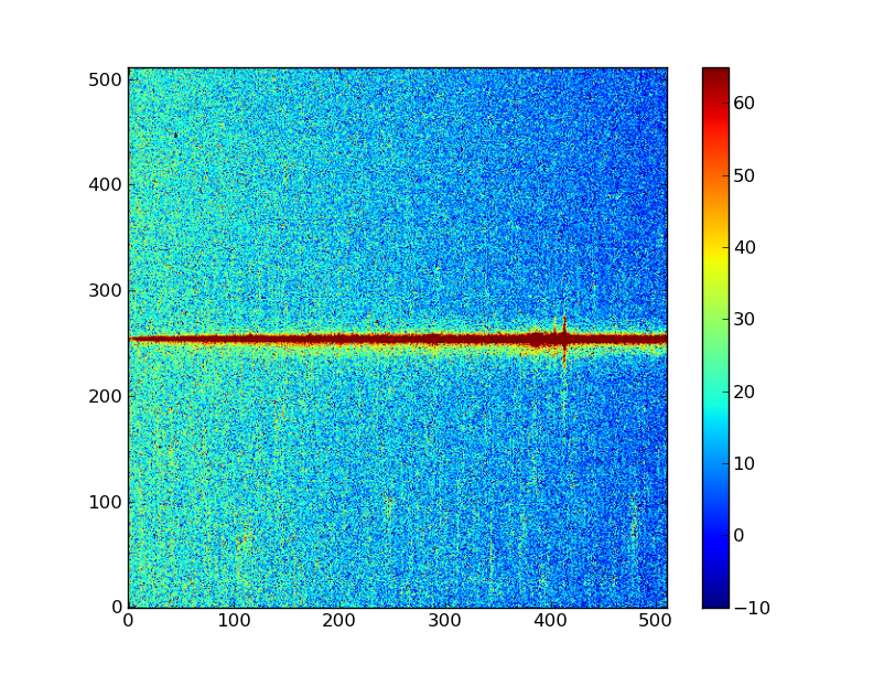
Next have a look at the images using one of the standard Matplotlib plotting functions. The slit (spatial) direction is along the rows (up and down) and wavelength is in columns (left to right).

plt.imshow(img)

You should see something resembling a horizontal line, but it will be difficult to make out much with the default settings. So, let’s set a few options for this plot. It’s not obvious from the data alone, but we want the origin in the lower left instead of the upper left corner. We also want to change the color scaling to something more sensible. By default, plt.imshow() scales the colors from the minimum to the maximum value in the data array that we pass it. In our case that is not the best option. We can set a lower and upper bound and add a colorbar to our plot:

plt.clf()
plt.imshow(img, origin = 'lower', vmin = -10, vmax = 65)
plt.colorbar()

Your plot should now look like something like what we show below. The colors may vary depending on your system’s settings.

Exercise: View the error and data quality images

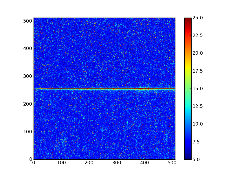
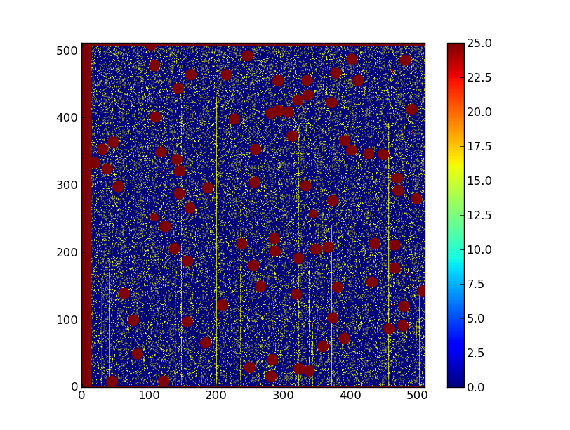
Bring up a viewer window for the other two images. Play with various buttons on the toolbar buttons and try to determine their functions. (Hint: imagine a web browser for the three on the left). Does the save button work for you?

Click here to show/hide solution

# Errors
plt.clf()
plt.imshow(err, origin = 'lower', vmin = 5, vmax = 25)
plt.colorbar()
# Data quality
plt.clf()
plt.imshow(dq, origin = 'lower', vmax = 25)
plt.colorbar()

Digging deeper in the 2D image

Now discover a little bit about the images you have read in, first with ?:

img?

If you get stuck with a colon (:) at the bottom of the screen without getting your prompt back, hit the q key. There is also a help function that gives you slightly different information:

help(img)

The same goes here: hit q to exit out of the display if you don’t get your prompt back. (This is called the “pager” and it follows the keys of the Unix more command.)

Finally, it is very important to get used to using “tab completion” to learn what you can do with your variables. At your IPython terminal, type img. without hitting Enter*, then hit the Tab key. You should see a table of names representing functions on the img variable. You can keep hitting Tab to cycle through the options, or use an arrow key to make the display go away. IPython is very smart and will give you helpful tab-completion suggestions for partial variable names, module names, functions, and more.

Finally let’s find the shape of the image and its minimum value:

img.shape  # Print the shape of img
img.min()  # Call the min() method on the img object.

NumPy basics

Before going further in our data analysis, we need to learn about a few key features of NumPy.

Making arrays

Recall that we said that the key feature of NumPy is that it lets us create variables containing multi-dimensional arrays of numbers. You can create these arrays in numerous ways. Below we show some examples. Here, the >>> prefix indicates a line that you could type into IPython, and any following lines without that prefix show what IPython will show you in response. You don’t have to type in these examples, but make sure to read them carefully.

>>> a = np.array([10, 20, 30, 40]) # create an array from a list of values
>>> a
array([10, 20, 30, 40]

>>> b = np.arange(4)  # create an array of 4 integers, from 0 to 3
>>> b
array([0, 1, 2, 3])

>>> np.arange(0.0, 10.0, 0.1)  # create an array from 0 to 100 stepping by 0.1
array([ 0. ,  0.1,  0.2,  0.3,  0.4,  0.5,  0.6,  0.7,  0.8,  0.9,  1. ,
        1.1,  1.2,  1.3,  1.4,  1.5,  1.6,  1.7,  1.8,  1.9,  2. ,  2.1,
        2.2,  2.3,  2.4,  2.5,  2.6,  2.7,  2.8,  2.9,  3. ,  3.1,  3.2,
        3.3,  3.4,  3.5,  3.6,  3.7,  3.8,  3.9,  4. ,  4.1,  4.2,  4.3,
        4.4,  4.5,  4.6,  4.7,  4.8,  4.9,  5. ,  5.1,  5.2,  5.3,  5.4,
        5.5,  5.6,  5.7,  5.8,  5.9,  6. ,  6.1,  6.2,  6.3,  6.4,  6.5,
        6.6,  6.7,  6.8,  6.9,  7. ,  7.1,  7.2,  7.3,  7.4,  7.5,  7.6,
        7.7,  7.8,  7.9,  8. ,  8.1,  8.2,  8.3,  8.4,  8.5,  8.6,  8.7,
        8.8,  8.9,  9. ,  9.1,  9.2,  9.3,  9.4,  9.5,  9.6,  9.7,  9.8,
        9.9])

>>> np.linspace(-np.pi, np.pi, 5)  # create an array of 5 evenly spaced samples from -pi to pi
array([-3.14159265, -1.57079633,  0.        ,  1.57079633,  3.14159265]))

New arrays can be obtained by operating with existing arrays. In NumPy, when you do math with arrays, it will do the math “elementwise,” by performing the requested operation on each array element separately. Continuing the above examples:

>>> a + b**2  # elementwise operations
array([10, 21, 34, 49])

Arrays may have more than one dimension:

>>> f = np.ones([3, 4])  # 3 x 4 array of ones
>>> f
array([[ 1.,  1.,  1.,  1.],
       [ 1.,  1.,  1.,  1.],
       [ 1.,  1.,  1.,  1.]])

Every element in an array must have the same “type”, but different arrays can be filled with different types. As is very common in computing, Python and NumPy distinguish between integer and “float” values. Integers (or just “ints”) can only take on integral values (fair enough), while ”floats” can approximate almost any real number. (“Float” is short for “floating-point,” which refers to the broad scheme by which non-integral values are encoded in binary. It is far beyond the purview of this tutorial, but every would-be scientific programmer must learn the basics of floating-point arithmetic.) In NumPy, each array has a “data type,” or dtype for short, that specifies the type of its contents:

>>> g = np.zeros([2, 3, 4], dtype=int)  # 2 x 3 x 4 integer array of zeros
array([[[0, 0, 0, 0],
        [0, 0, 0, 0],
        [0, 0, 0, 0]],
       [[0, 0, 0, 0],
        [0, 0, 0, 0],
        [0, 0, 0, 0]]])

>>> i = np.zeros_like(f)  # array of zeros with same shape and type as "f"
array([[ 0.,  0.,  0.,  0.],
       [ 0.,  0.,  0.,  0.],
       [ 0.,  0.,  0.,  0.]]))

You can change the dimensions of existing arrays, including changing the number of dimensions that they have:

>>> w = np.arange(12)
>>> w.shape = [3, 4]  # does not modify the total number of elements
array([[ 0,  1,  2,  3],
       [ 4,  5,  6,  7],
       [ 8,  9, 10, 11]])

>>> x = np.arange(5)
>>> x
array([0, 1, 2, 3, 4])

>>> y = x.reshape(5, 1)
>>> y = x.reshape(-1, 1)  # Same thing but NumPy figures out correct length
>>> y
array([[0],
       [1],
       [2],
       [3],
       [4]]))

It is possible to operate with arrays of different dimensions as long as they fit “well”. NumPy does this using a paradigm called broadcasting. In short, NumPy will almost always “do what you want” without needing any tricks. But frequent NumPy users should read the rules of broadcasting to make sure they understand how the system works.

>>> x.shape
(5,)
>>> y.shape
(5, 1)
>>> x + y * 10
array([[ 0,  1,  2,  3,  4],
       [10, 11, 12, 13, 14],
       [20, 21, 22, 23, 24],
       [30, 31, 32, 33, 34],
       [40, 41, 42, 43, 44]])

Exercise: Make a ripple

Set x to an array that goes from -20 to 20, stepping by 0.25. Make y the same as x but “transposed” using the reshape trick above. Calculate a surface z = cos(r) / (r + 5) where r = sqrt(x**2 + y**2). Use plt.imshow to display the image of z.

Click here to show/hide solution

x = np.arange(-20, 20, 0.25)
y = x.reshape(-1, 1)
r = np.sqrt(x**2 + y**2)
z = np.cos(r) / (r + 5)
plt.imshow(z, origin = 'lower)

Array access and slicing

NumPy provides powerful methods for accessing array elements or particular subsets of an array, e.g. “the fourth column” or “every other row.” This is called “slicing.” The outputs below illustrate basic slicing. Once again you don’t need to type these examples, but you should read them carefully:

>>> a = np.arange(20).reshape(4,5)
>>> a
array([[ 0,  1,  2,  3,  4],
      [ 5,  6,  7,  8,  9],
      [10, 11, 12, 13, 14],
      [15, 16, 17, 18, 19]])

>>> a[2, 3]  # select element in row 2, column 3 (counting from 0)
13

>>> a[2, :]  # select every element in row 2
array([10, 11, 12, 13, 14])

>>> a[:, 0]  # select every element in column 0
array([ 0,  5, 10, 15])

>>> a[2, 0:4]  # select columns 0 to *3* in row 2
array([10, 11, 12, 13])

>>> a[0:3, 1:3] # select a sub-matrix.
array([[ 1,  2],
       [ 6,  7],
       [11, 12]])

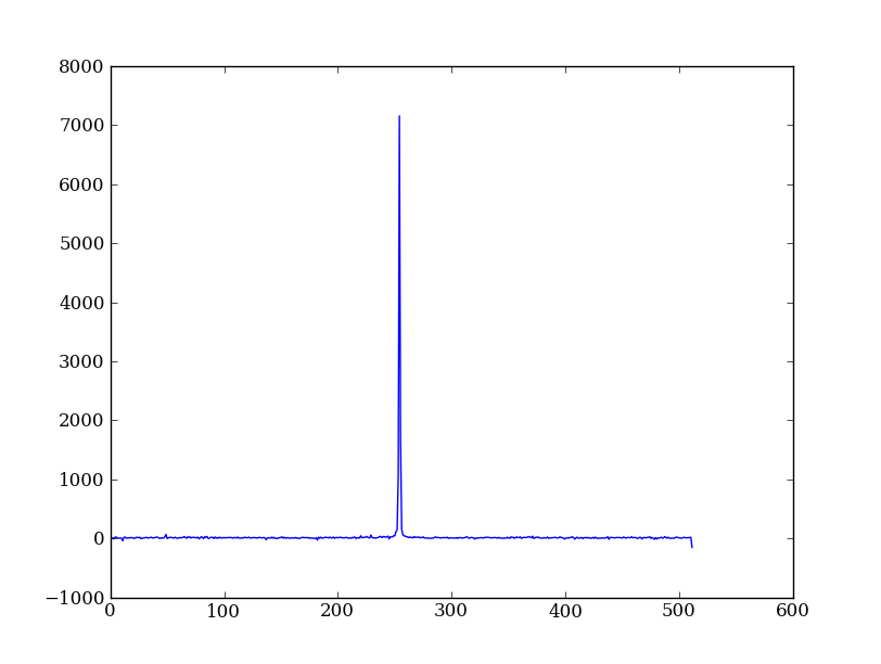
As a first practical example, let’s plot column 300 of the STIS long-slit image to look at the spatial profile:

plt.figure()  # Start a new plot -- by default matplotlib overplots.
plt.plot(img[:, 300])

The formal syntax for array slicing is as follows. For each dimension of an array, the most general “slice” that you can write has the form:

I0:I1:STEP

Where

• I0 is the first index value. This can be any Python expression that works out to an integer, or you can leave it blank to default to 0.
• I1 is the index upper bound. Once again this can be any Python expression. If you leave it blank, the slicing goes until the end of the axis.
• STEP is the “step size” between each successive index. The default is one. When step is not specified then the final : is not required.

The number one “gotcha” about slicing is that the I1-th index is not included in your slice. For instance, the slice 1:3 selects only two elements. The slice 3:3 selects zero array elements (which is perfectly allowed). This definition is counterintuitive for most people, but it has its merits. For instance, the number of elements in a slice is exactly I1 - I0 (unless STEP is not 1). And the slices X:Y and Y:Z are non-overlapping subsets of the slice X:Z.

To slice an array along multiple dimensions at once, you just separate different slices with commas, writing something along the lines of:

array[SLICE0, SLICE1, ...]

Where SLICE0 stands for one of the expressions described above, and so on.

There are other special cases to slicing: negative indices have special meaning, for instance. TODO: point to comprehensive documentation! I can‘t find any!

Exercise: Slice the error array

• Starting with column 10 and ending at column 200, plot every third column of row 254 of the error array err.
• Print out the numbers in a rectangular sub-matrix of the data quality array dq with rows 251 to 253 (inclusive) and columns 101 to 104 (inclusive). What did you learn about the index upper bound value?

Click here to show/hide solution

plt.clf()
plt.plot(err[254, 10:200:3])
dq[251:254, 101:105]

The index upper bound I1 is one more than the final index that gets included in the slice. In other words the slice includes everything up to, but not including, the index upper bound I1. There are good reasons for this, but for now just accept and learn it.

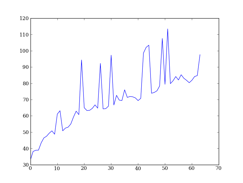
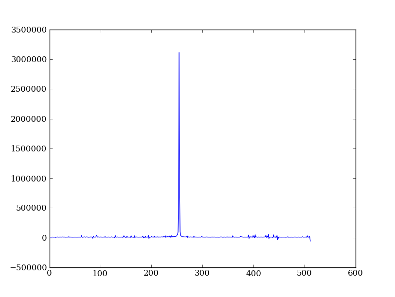
Plot the spatial profile and raw spectrum

Plot the spatial profile by summing along the wavelength direction:

profile = img.sum(axis=1)
plt.figure()
plt.plot(profile)

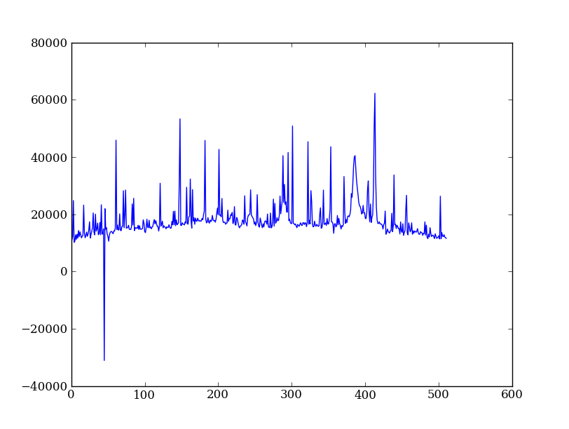
Now plot the spectrum by summing along the spatial direction:

spectrum = img.sum(axis=0)
plt.figure()
plt.plot(spectrum)

Since most of the sum is in the background region there is a lot of noise and cosmic-ray contamination.

Exercise: Use slicing to make a better spectrum plot

Use slicing to do the spectrum sum using only the rows in the image where there is a signal from the source. Hint: zoom into your profile plot to find a reasonable range of rows to use.

Click here to show/hide solution

Here’s one suggested row range:

spectrum = img[250:260, :].sum(axis=0)
plt.clf()
plt.plot(spectrum)

Filter cosmic rays from the background

Let’s plot five columns from the spectrum image as follows. Recall that each column is a cut along the spatial direction; so we’re isolating the data from five adjacent wavelength bins:

plt.clf()
plt.plot(img[:, 254:259])

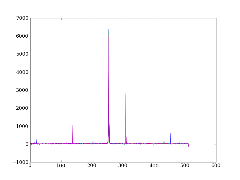
The basic goal of two-dimensional spectral extraction is to subtract out the background and sum over the rows with the source signal.

The big spikes in the plot you just made are showing that there are significant cosmic ray defects in the data. In order to do a good job of subtracting the background we need to filter them out. Doing this correctly in general is difficult, and for real work we’d just use the answers already provided by the Hubble data analysts. But let’s pretend that we have to do the cosmic-ray filtering ourselves.

A simple strategy to accomplish this is to use a median filter to smooth out single-pixel deviations. Then we can use sigma-clipping to remove large variations between the actual and smoothed image. We will leverage existing routines in the SciPy signal processing module to accomplish this:

import scipy.signal
img_sm = scipy.signal.medfilt(img, 5)
sigma = np.median(err)
bad = (np.abs(img - img_sm) / sigma) > 8.0
img_cr = img.copy()
img_cr[bad] = img_sm[bad]
img_cr[230:280,:] = img[230:280,:]  # Filter only for background

Let’s check if it worked by making the same plot as before, but using the filtered data

plt.clf()
plt.plot(img_cr[:, 254:259])

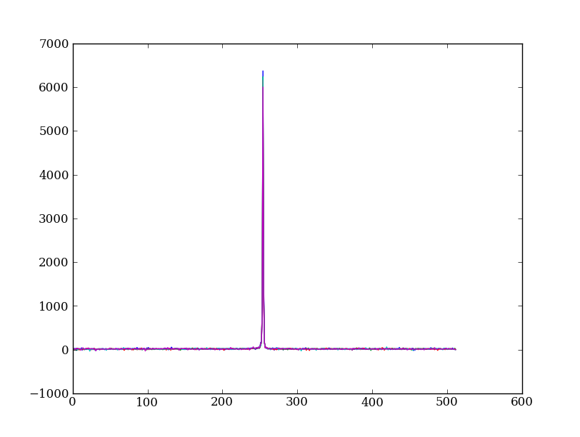
Above we used an important NumPy tool: indexing an array with a boolean mask. Let’s look at a smaller example:

>>> a = np.array([1, 4, -2, 4, -5])
>>> neg = (a < 0)  # Parentheses here for clarity but are not required
>>> neg
array([False, False,  True, False,  True], dtype=bool)

>>> a[neg] = 0
>>> a
array([1, 4, 0, 4, 0])

A slightly more complex example shows that this works the same on multi-dimensional arrays, and that you can compose logical expressions:

>>> a = np.arange(25).reshape(5,5)
>>> ok = (a > 6) & (a < 17)  # "ok = a > 6 & a < 17" will FAIL!
>>> a[~ok] = 0  # "~" is the "logical not" operator
>>> a
array([[ 0,  0,  0,  0,  0],
       [ 0,  0,  7,  8,  9],
       [10, 11, 12, 13, 14],
       [15, 16,  0,  0,  0],
       [ 0,  0,  0,  0,  0]])

Exercise [intermediate]: circular region slicing

Remember the surface z = cos(r) / (r + 5) that you made previously. Set z = 0 for every pixel of z that is within 10 units of (x,y) = (10, 15).

Click here to show/hide solution

dist = np.sqrt((x-10)**2 + (y-15)**2)
mask = dist < 10
z[mask] = 0
plt.imshow(z, origin = 'lower')

Detour: copy versus reference

Question

In the median filtering commands above we wrote img_cr = img.copy(). Why was that needed instead of just img_cr = img?

Answer

Because the statement img_cr = img would just create another reference pointing to the underlying array object that img references. In other words, all it would do is give you another name by which to access for the same block of data.

Variable names in Python are just “pointers” to actual Python objects. To see this clearly do the following:

>>> a = np.arange(8)
>>> b = a
>>> id(a)  # Unique identifier for the object referred to by "a"
122333200

>>> id(b)  # Unique identifier for the object referred to by "b"
122333200

>>> b[3] = -10  # Modifying "b" modifies "a" too!
>>> a
array([  0,   1,   2, -10,   4,   5,   6,   7])

After getting over the initial confusion this behavior is actually a good thing because it is efficient and consistent within Python. If you really need a copy of an array then use the copy() method as shown.

BEWARE of one common pitfall: “basic” slicing in NumPy, like a[3:6], does not make copies:

>>> b = a[3:6]
>>> b
array([-10,   4,   5])

>>> b[1] = 100
>>> a
array([  0,   1,   2, -10, 100,   5,   6,   7])

However if you do arithmetic or boolean mask then a copy is always made:

>>> a = np.arange(4)
>>> b = a**2
>>> a[1] = 100
>>> a
array([  0, 100,   2,   3])

>>> b  # Still as expected after changing "a"
array([0, 1, 4, 9])

Fit the background

To subtract the background signal from the source region we want to fit a quadratic to the background pixels, then subtract that quadratic from the entire image — including the source region.

Let’s tackle a simpler problem first and fit the background for a single column. From visual inspection of the 2D spectrum, we have decided to isolate rows 10–199 and 300–479 as ones containing pure background signal:

x = np.append(np.arange(10, 200), np.arange(300, 480))  # Background rows
y = img_cr[x, 10]  # Background rows in column 10 of cleaned image
plt.figure()
plt.plot(x, y)
pfit = np.polyfit(x, y, 2)  # Fit a 2nd order polynomial to (x, y) data
yfit = np.polyval(pfit, x)  # Evaluate the polynomial at x
plt.plot(x, yfit)
plt.grid()

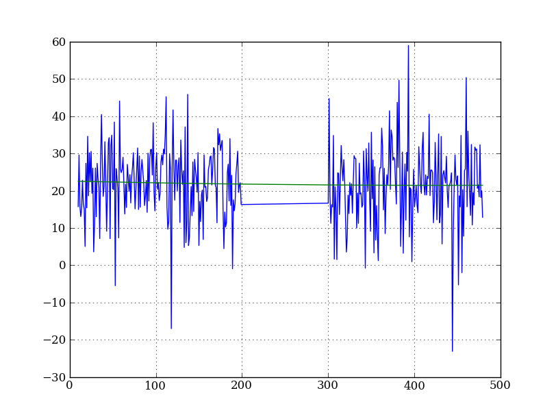
Now let’s do this for every column and store the results in a background image:

xrows = np.arange(img_cr.shape[0])          # Array from 0 .. N_rows-1
bkg = np.zeros_like(img_cr)                 # Empty image for background fits
for col in np.arange(img_cr.shape[1]):      # For each column ...
    pfit = np.polyfit(x, img_cr[x, col], 2) # Fit poly over bkg rows for col
    bkg[:, col] = np.polyval(pfit, xrows)   # Eval poly at ALL row positions

plt.clf()
plt.imshow(bkg, origin = 'lower', vmin=0, vmax=20)
plt.colorbar()

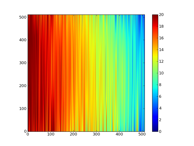
Finally let’s subtract this background and see how the results look:

img_bkg = img_cr - bkg
plt.clf()
plt.imshow(img_bkg, origin = 'lower', vmin=0, vmax=60)
plt.colorbar()

Background subtracted	Original

Detour: vector operations versus looping

If you are used to C or Fortran you might be wondering why jump through these hoops with slicing and making sure everything is vectorized. The answer is that pure Python is an interpreted dynamic language and hence doing loops is slow. Try the following:

size = 500000
x = np.arange(size)
a = np.zeros(size)
%time for i in x: a[i] = x[i] / 2.0

Now compare to the vectorized NumPy solution:

x = np.arange(size)
%time a = x / 2

Sometimes doing things in a vectorized way is not possible or just too confusing. There is an art here and the basic answer is that if it runs fast enough then you are good to go. Otherwise things need to be vectorized or maybe coded in C or Fortran.

Sum the source signal

The final step in our analysis is to sum up the remaining source signal across rows to obtain a one-dimensional spectrum. We leave this as an exercise!

Python for Astronomers Spectrum	HST official spectrum

The biggest difference between our result and the official HST result is that they have flux-calibrated the instrument’s response as a function of wavelength. We haven’t bothered to do that here.

Exercise: Make the final spectrum

Take the background-subtracted spectrum, sum up the rows containing the astronomical signal, and plot the resulting one-dimensional spectrum. You’ve already done this step in a previous exercise, but it was just using the un-corrected data.

Click here to show/hide solution

spectrum = img_bkg[250:260, :].sum(axis=0)
plt.clf()
plt.plot(spectrum)

Next steps

There is much more to do and learn! We have omitted many important details in this crash course, and there are literally thousands of features in the astronomical Python toolkit that we haven’t even mentioned. Just take a quick look at the tables of contents for the SciPy Reference Manual or the AstroPy documentation to get a sense of how much is available.