Tabular data
Astropy includes a class for representing arbitrary tabular data in
astropy.table, called Table. This class can be imported with:
from astropy.table import Table
You may need to also import the Column class, depending on how you are
definining your table (see below):
from astropy.table import Table, Column
Documentation
For more information about the features presented below, you can read the astropy.table docs.
Constructing and Manipulating tables
There are a number of ways of constructing tables. One simple way is to start from existing lists or arrays:
>>> from astropy.table import Table
>>> a = [1, 4, 5]
>>> b = [2.0, 5.0, 8.2]
>>> c = ['x', 'y', 'z']
>>> t = Table([a, b, c], names=('a', 'b', 'c'))
There are a few ways to examine the table. You can get detailed information about the table values and column definitions as follows:
>>> t
<Table rows=3 names=('a','b','c')>
array([(1, 2.0, 'x'), (4, 5.0, 'y'), (5, 8.2, 'z')],
      dtype=[('a', '<i8'), ('b', '<f8'), ('c', '|S1')])
If you print the table (either from the noteboook or in a text console session) then a formatted version appears:
>>> print(t)
  a   b   c
--- --- ---
  1 2.0   x
  4 5.0   y
  5 8.2   z
Now examine some high-level information about the table:
>>> t.colnames
['a', 'b', 'c']

>>> len(t)
3
Access the data by column or row using the same syntax as for Numpy structured arrays:
>>> t['a']       # Column 'a'
<Column name='a' units=None format=None description=None>
array([1, 4, 5])

>>> t['a'][1]    # Row 1 of column 'a'
4

>>> t[1]         # Row obj for with row 1 values
<Row 1 of table
  values=(4, 5.0, 'y')
  dtype=[('a', '<i8'), ('b', '<f8'), ('c', '|S1')]>

>>> t[1]['a']    # Column 'a' of row 1
4
One can retrieve a subset of a table by rows (using a slice) or columns (using column names), where the subset is returned as a new table:
>>> print(t[0:2])      # Table object with rows 0 and 1
 a   b   c
--- --- ---
  1 2.0   x
  4 5.0   y

>>> t['a', 'c']  # Table with cols 'a', 'c'
 a   c
--- ---
  1   x
  4   y
  5   z
Modifying table values in place is flexible and works as one would expect:
>>> t['a'] = [-1, -2, -3]       # Set all column values
>>> t['a'][2] = 30              # Set row 2 of column 'a'
>>> t[1] = (8, 9.0, "W")        # Set all row values
>>> t[1]['b'] = -9              # Set column 'b' of row 1
>>> t[0:2]['b'] = 100.0         # Set column 'c' of rows 0 and 1
>>> print(t)
 a    b    c
--- ----- ---
 -1 100.0   x
  8 100.0   W
 30   8.2   z
Add, remove, and rename columns with the following:
>>> t.add_column(Column(data=[1, 2, 3], name='d')))
>>> t.remove_column('c')
>>> t.rename_column('a', 'A')
>>> t.colnames
['A', 'b', 'd']
Adding a new row of data to the table is as follows:
>>> t.add_row([-8, -9, 10])
>>> len(t)
4
Lastly, one can create a table with support for missing values, for example by setting
masked=True:
>>> t = Table([a, b, c], names=('a', 'b', 'c'), masked=True)
>>> t['a'].mask = [True, True, False]
>>> t
<Table rows=3 names=('a','b','c')>
masked_array(data = [(--, 2.0, 'x') (--, 5.0, 'y') (5, 8.2, 'z')],
             mask = [(True, False, False) (True, False, False) (False, False, False)],
       fill_value = (999999, 1e+20, 'N'),
            dtype = [('a', '<i8'), ('b', '<f8'), ('c', '|S1')])

>>> print(t)
 a   b   c
--- --- ---
 -- 2.0   x
 -- 5.0   y
  5 8.2   z
Finally, every table can have meta-data attached to it via the meta
attribute, which can be used like a Python dictionary:
>>> t.meta['creator'] = 'me'
Reading and writing tables
Table objects include read and write methods that can be used to
easily read and write the tables to different formats. The tutorial directory
contains a file named rosat.vot which is the ROSAT All-Sky Bright Source
Catalogue (1RXS) (Voges+ 1999) in the VO Table format.
You can read this in as a Table object by simply doing:
>>> t = Table.read('rosat.vot', format='votable')
(just ignore the warnings, which are due to Vizier not complying with the VO standard). We can see a quick overview of the table with:
>>> print(t)
     _1RXS        RAJ2000   DEJ2000  PosErr NewFlag   Count    e_Count   HR1  e_HR1  HR2  e_HR2 Extent
---------------- --------- --------- ------ ------- --------- --------- ----- ----- ----- ----- ------
J000000.0-392902   0.00000 -39.48403     19    __..      0.13     0.035  0.69  0.25  0.28  0.24      0
J000007.0+081653   0.02917   8.28153     10    TT..      0.19     0.021  0.89  0.10  0.24  0.13      0
J000010.0-633543   0.04167 -63.59528     11    __..      0.19     0.031 -0.36  0.13 -0.35  0.23     13
J000011.9+052318   0.04958   5.38833      7    __..      0.26     0.026  0.24  0.10  0.00  0.13      0
J000012.6+014621   0.05250   1.77250     11    __..     0.081     0.016  0.05  0.20  0.00  0.26     14
J000013.5+575628   0.05625  57.94125      8    __..      0.12     0.017  0.57  0.12  0.32  0.14      0
J000019.5-261032   0.08125 -26.17556     12    __..      0.12     0.022 -0.26  0.17  0.19  0.29      0
             ...       ...       ...    ...     ...       ...       ...   ...   ...   ...   ...    ...
J235929.2-255851 359.87164 -25.98083     10    _T..      0.23     0.028 -0.43  0.11 -0.30  0.26     13
J235929.3+334329 359.87207  33.72472     11    __..      0.16     0.024 -0.62  0.12 -0.56  0.66     12
J235930.9-401541 359.87875 -40.26139     18    __..      0.13     0.037 -0.73  0.18  0.02  0.82      0
J235940.9-314342 359.92041 -31.72847     19    __..     0.058     0.017  0.17  0.30  0.33  0.34      0
J235941.2+830719 359.92166  83.12195     10    __..     0.066     0.011  0.72  0.14  0.19  0.17      0
J235944.7+220014 359.93625  22.00389     17    __..     0.052     0.015 -0.01  0.27  0.37  0.35      0
J235959.1+083355 359.99625   8.56528     10    __..      0.12     0.018  0.54  0.13  0.10  0.17      9
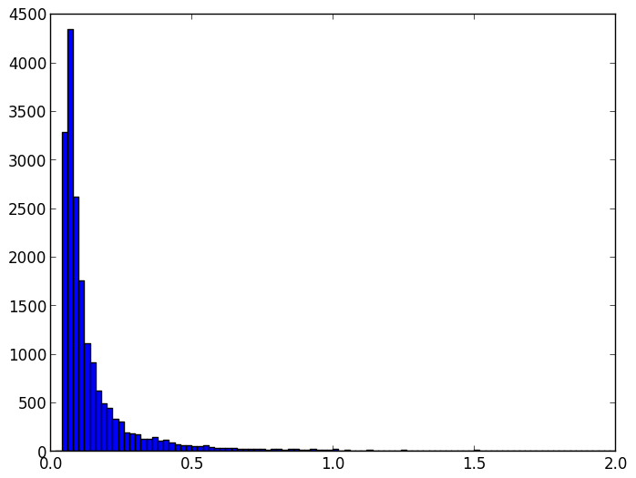
Since we are using IPython with the --matplotlib option along with
import matplotlib.pyplot as plt, we can easily make a
histogram of the count rates:
>>> plt.hist(t['Count'], range=[0., 2], bins=100)
It is easy to select a subset of the table matching a given criterion:
>>> t_bright = t[t['Count'] > 0.2]
>>> len(t_bright)
3627
Criteria can be combined:
>>> t_sub = t[(t['RAJ2000'] > 230.) & (t['RAJ2000'] < 260.) &
              (t['DEJ2000'] > -60.) & (t['DEJ2000'] < -20)]

>>> len(t_sub)
642
Practical Exercises
Excercise
Try and find a way to make a table of the ROSAT point source catalog that
contains only the RA, Dec, and count rate. Hint: you can see what methods
are available on an object by typing e.g. t. and then pressing
<TAB>. You can also find help on a method by typing e.g.
t.add_column?.
Click to Show/Hide Solution
>>> t.keep_columns(['RAJ2000', 'DEJ2000', 'Count'])
>>> print(t)
 RAJ2000   DEJ2000    Count
--------- --------- ---------
  0.00000 -39.48403      0.13
  0.02917   8.28153      0.19
  0.04167 -63.59528      0.19
  0.04958   5.38833      0.26
  0.05250   1.77250     0.081
  0.05625  57.94125      0.12
  0.08125 -26.17556      0.12
      ...       ...       ...
359.87207  33.72472      0.16
359.87875 -40.26139      0.13
359.92041 -31.72847     0.058
359.92166  83.12195     0.066
359.93625  22.00389     0.052
359.99625   8.56528      0.12

Note that you can also do this with::

>>> t_new = t['RAJ2000', 'DEJ2000', 'Count']
>>> print(t_new)
 RAJ2000   DEJ2000    Count
--------- --------- ---------
  0.00000 -39.48403      0.13
  0.02917   8.28153      0.19
  0.04167 -63.59528      0.19
  0.04958   5.38833      0.26
  0.05250   1.77250     0.081
  0.05625  57.94125      0.12
  0.08125 -26.17556      0.12
      ...       ...       ...
359.87207  33.72472      0.16
359.87875 -40.26139      0.13
359.92041 -31.72847     0.058
359.92166  83.12195     0.066
359.93625  22.00389     0.052
359.99625   8.56528      0.12
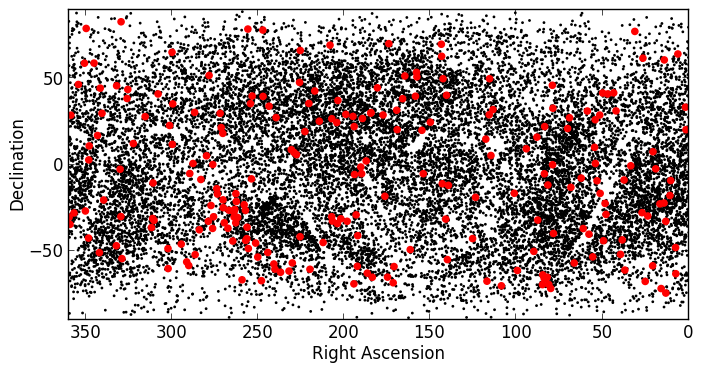
Excercise 2
Make an all-sky equatorial plot of the ROSAT sources, with all sources shown in black, and only the sources with a count rate larger than 2. shown in red.
Click to Show/Hide Solution
from astropy.table import Table
from matplotlib import pyplot as plt

t = Table.read('rosat.vot', format='votable')
t_bright = t[t['Count'] > 2.]

fig = plt.figure()
ax = fig.add_subplot(1,1,1, aspect='equal')
ax.scatter(t['RAJ2000'], t['DEJ2000'], s=1, color='black')
ax.scatter(t_bright['RAJ2000'], t_bright['DEJ2000'], color='red')
ax.set_xlim(360., 0.)
ax.set_ylim(-90., 90.)
ax.set_xlabel("Right Ascension")
ax.set_ylabel("Declination")

fig.savefig('tables_level2.png', bbox_inches='tight')
Excercise 3
Try and write out the ROSAT catalog into a format that you can read into another software package (see here for more details). For example, try and write out the catalog into CSV format, then read it into a spreadsheet software package (e.g. Excel, Google Docs, Numbers, OpenOffice).
Click to Show/Hide Solution
To write out the file:
>>> t.write('rosat2.csv', format='ascii', delimiter=',')
Then you should be able to load it into another software package.